What is a Loss Function?
How to formulate the right objective.

Any machine learning student will learn about loss functions sooner rather than later. They are a fundamental element of learning and optimisation, therefore understanding is necessary for mastering machine learning. At its heart it is a simple concept, however, a quick search in google gives you a convoluted Wikipedia definition.
“A function that maps an event or values of one or more variables onto a real number intuitively representing some “cost” associated with the event” - Wikipedia
To decipher the definition we will take a more general perspective, not limiting ourselves just to machine learning. We will then discuss two basic loss functions used in machine learning to understand where they come from and what they imply.
The General Perspective
Loss functions are a mathematical formulation of a problem that we are trying to solve. They describe our goal or objective. The function at any given time will tell us how close we are to reaching the objective. An important feature of loss functions is that they will also tell you how to reach the objective. We will look at a couple of examples where we might use loss functions in our daily lives.
Costs vs Income
Say you run a company. However, you are in the red and your investors tell you to minimize losses. You measure your costs and incomes and write down the difference, which is your loss. \begin{equation*} loss = costs - income \end{equation*} Your objective is to minimize your company’s loss and you can now measure how big is the loss. Now if you see that the output of this function decreases that means you are on the right track, but if it increases then you are getting further away from your goal. The loss function also tells you which actions to take to succeed. You can see that you need to decrease costs and increase income.
This formulation is the standard for loss functions, we will have some costs and some benefits, which together will give you a performance measure. Sometimes they may be called punishments and rewards. In this example, we are punishing costs and rewarding income.
Fencing a vegetable garden
Let’s now look at a classical optimisation problem. Imagine you want to fence out a rectangle plot in your garden to grow vegetables. You need $4 \text{ m}^2$ of land to fit everything you need, but you need to build a fence to keep your cat from ruining your crops. However, you want to spend as little money as possible.
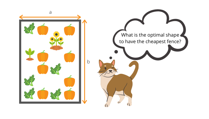
This is an optimisation problem, where your goal is to find the minimal circumference for the given area. Therefore the circumference is our loss function: \begin{align*} C &= 2 (a + b) \newline &= 2b\left(P^{-1} + 1\right) \end{align*} The larger the circumference the worse the shape is (the more it will cost you to build the fence). To find the optimal solution under the area ($P$) constraint we need to compute the derivative of the loss function and solving it will give us the solution: \begin{equation*} a = b = \sqrt{P} = 2 \text{ m} \end{equation*} We use loss functions analogously in machine learning, however for optimising we might prefer using a numerical method like gradient descent. To use a loss function properly we need to know the objective.
Objectives in Machine Learning
- Regression: Predict the values as well as possible.
- Classification: Assign the best class to values.
- Reinforcement: Get the most reward.
- Clustering: Discover relations in the data.
In this post, we will focus on loss functions for regression as these are the simplest to understand. We will look into the other loss functions another time.
A measure of distance
The key idea is to measure the distance between the ground truth and the model. Let’s imagine that our data consists of two points: $y(x_1) = 2$ and $y(x_2) = 2$. We can plot this on a coordinate system as a point $(2, 2)$. This is visualised on the plot below as the black dot.
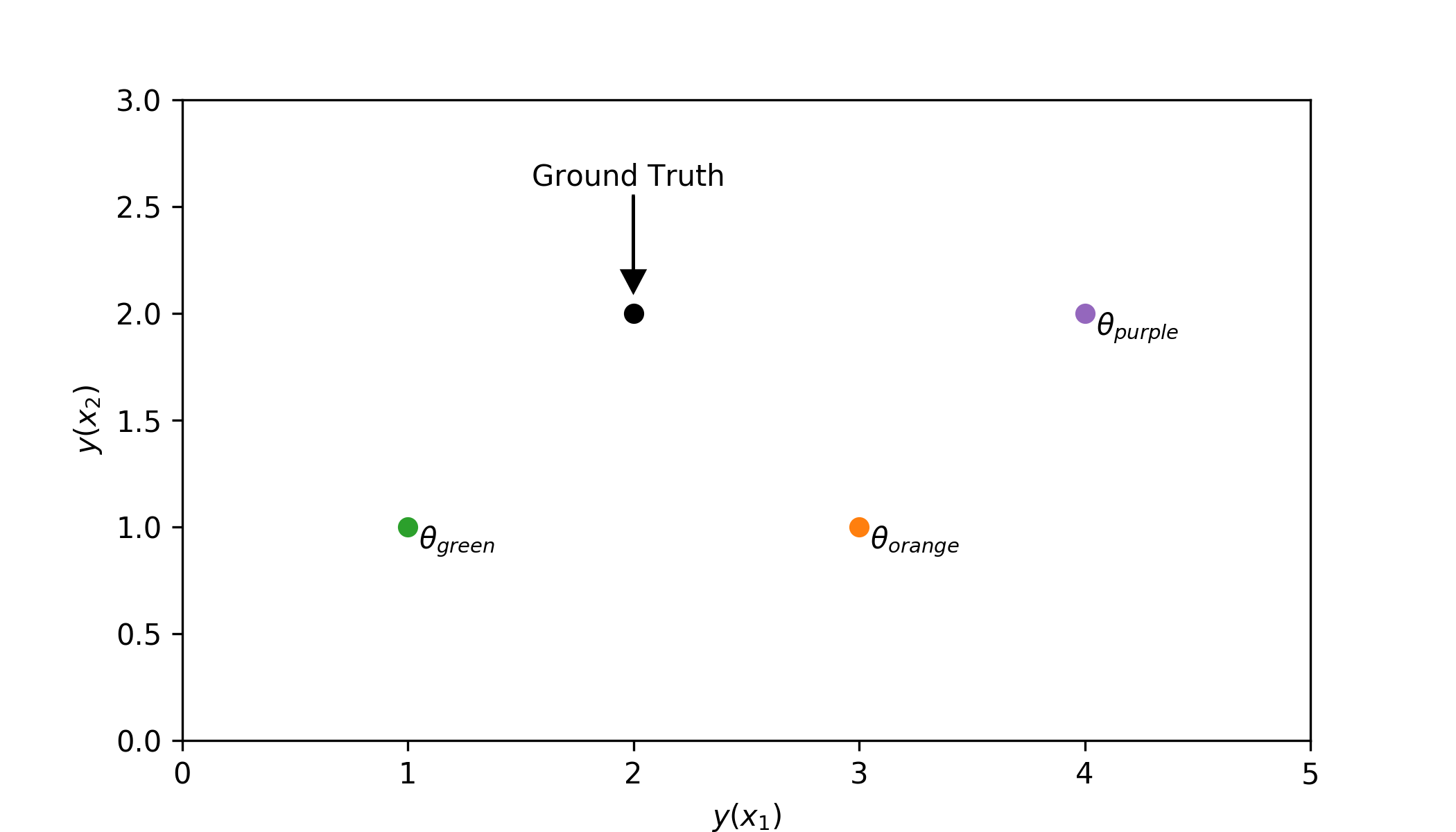
We now define a model $\hat{y}(x_n, \theta)$. The $\theta$ represents the set of parameters of the model, which will determine it’s output. Let’s say we have models which predict:
- $\hat{y}(x_n; \theta_{green}) \rightarrow (1, 1)$
- $\hat{y}(x_n; \theta_{orange}) \rightarrow (3, 1)$
- $\hat{y}(x_n; \theta_{purple}) \rightarrow (4, 2)$
They have been marked on the figure above using green, orange and purple dots. Now you have to decide which model is better: the green, orange or the purple one?
The perfect model would predict the same values as the ground truth, meaning it would be in the same position as the black dot. (This does not necessarily mean that it will be the best prediction. See: Overfitting) This means that $y(x_n) = \hat{y}(x_n; \theta)$ and that their difference is equal to $0$.
\begin{equation*} \delta(x_n; \theta) = \hat{y}(x_n; \theta) - y(x_n) \end{equation*}
However, just subtracting the ground truth from the model will not result in a scalar. So we will sum the differences to get a single value. Let’s see what are the results.
| model | prediction | $\sum_n \delta(x_n, \theta)$ |
|---|---|---|
| perfect | $(2, 2)$ | $0$ |
| green | $(1, 1)$ | $-2$ |
| orange | $(3, 1)$ | $\mathbf{0}$ |
| purple | $(4, 2)$ | $2$ |
Unfortunately, there is a problem with this method. It suggests that the orange model would be the best. It says that it is equally as good as the perfect model, which you can see is not true. Also, we have both positive and negative values, which doesn’t aid in the interpretation of how good each model is. This is primarily because \begin{equation}\label{eq:l_non} L(\theta) = \sum_n^N \delta(x_n; \theta) \end{equation} is not a metric. So this is an incorrect method of measuring distances between points. However, this does provide a good basis for understanding the metrics that we will discuss next.
Mean Absolute Error, L1 Loss
This method uses the L1 norm as a measure of distance otherwise known as the Taxicab metric. It measures the distance as if we moved in a grid-like space. A visualisation of this is shown below.
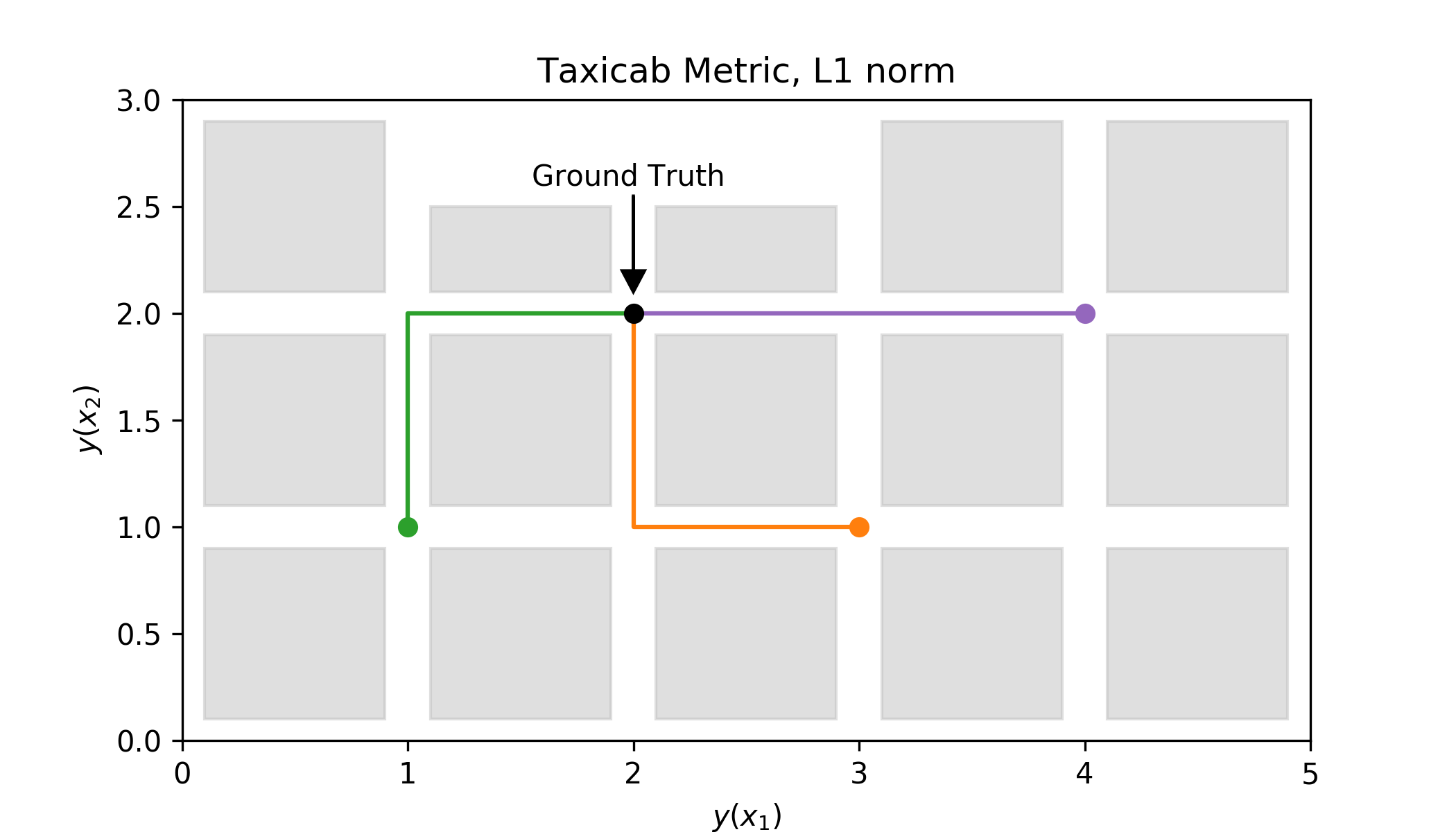
Mathematically this is expressed using the absolute value (hence L1-norm as the polynomial order is 1). As a result we modify equation \ref{eq:l_non} to be \begin{equation*} L(\theta) = \sum_n^N |\delta(x_n; \theta)| \end{equation*} We will also divide by $N$ to make the distance independent from the number of data points. This will essentially give us the mean distance. \begin{equation}\label{eq:mae} L(\theta) = \frac{1}{N}\sum_n^N |\delta(x_n; \theta)| \end{equation}
Now let’s apply this to the example models and let’s see which model is the best according to this loss function. The table below shows you the distances for each model.
| model | prediction | L1 norm |
|---|---|---|
| perfect | $(2, 2)$ | $0$ |
| green | $(1, 1)$ | $2$ |
| orange | $(3, 1)$ | $2$ |
| purple | $(4, 2)$ | $2$ |
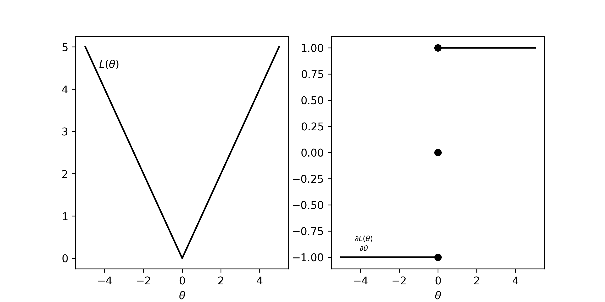
As you may realise based on this distance metric all of the models are equally good (or bad). But how can we find better parameters for our models? Since we want to find the $\theta$ which minimizes this loss function we can use gradient descent. In order to do this we need to calculate the gradient. \begin{equation*} \frac{\partial L(\theta)}{\partial \theta} = \frac{1}{N} \sum_{n=1}^N \text{sgn}\big(\delta(x_n; \theta)\big)\frac{\partial \hat{y}}{\partial \theta} \end{equation*} Where $\text{sgn}(\cdot)$ is the sign function, which is equal to $1$ for positive inputs and $-1$ for negative inputs. This is a slight inconvenience as the gradient is not continuous making it more computationally expensive to compute. Furthermore, the gradient is constant (for positive or negative errors) and as a result, it is more difficult to converge to the minimum. Traces of the loss function and derivative are shown in the figure below.
The python implementation is rather straightforward.
1
2
3
4
5
def mae(y_pred, y_true):
    return np.mean(np.abs(y_pred - y_true))

def mae_grad(y_pred, y_true, y_pred_grad):
    return np.mean(np.sign(y_pred - y_true) * y_pred_grad)
You can find an interactive demo below. The goal is to fit the line on the right to the data (green dots) by changing the $\theta$ slider. You can change the amount of data that you need to fit the model by moving the $N$ slider. The left plot shows you the loss function. You can see how it changes with the increased amount of data and that the minimum will give you a good fit to the data. What happens when you fit perfectly to one point and then start to add more data? Does the fit remain good?
Next, we will look at a slightly different approach, which can help solve some of the problems introduced by the mean absolute error.
Mean Squared Error, L2 Loss
In the second method, we will use a different metric. Here we will depend on the L2 norm otherwise known as the Euclidean Metric. It measures the distance as if you could get everywhere by following a straight line. You can find a visualisation below.
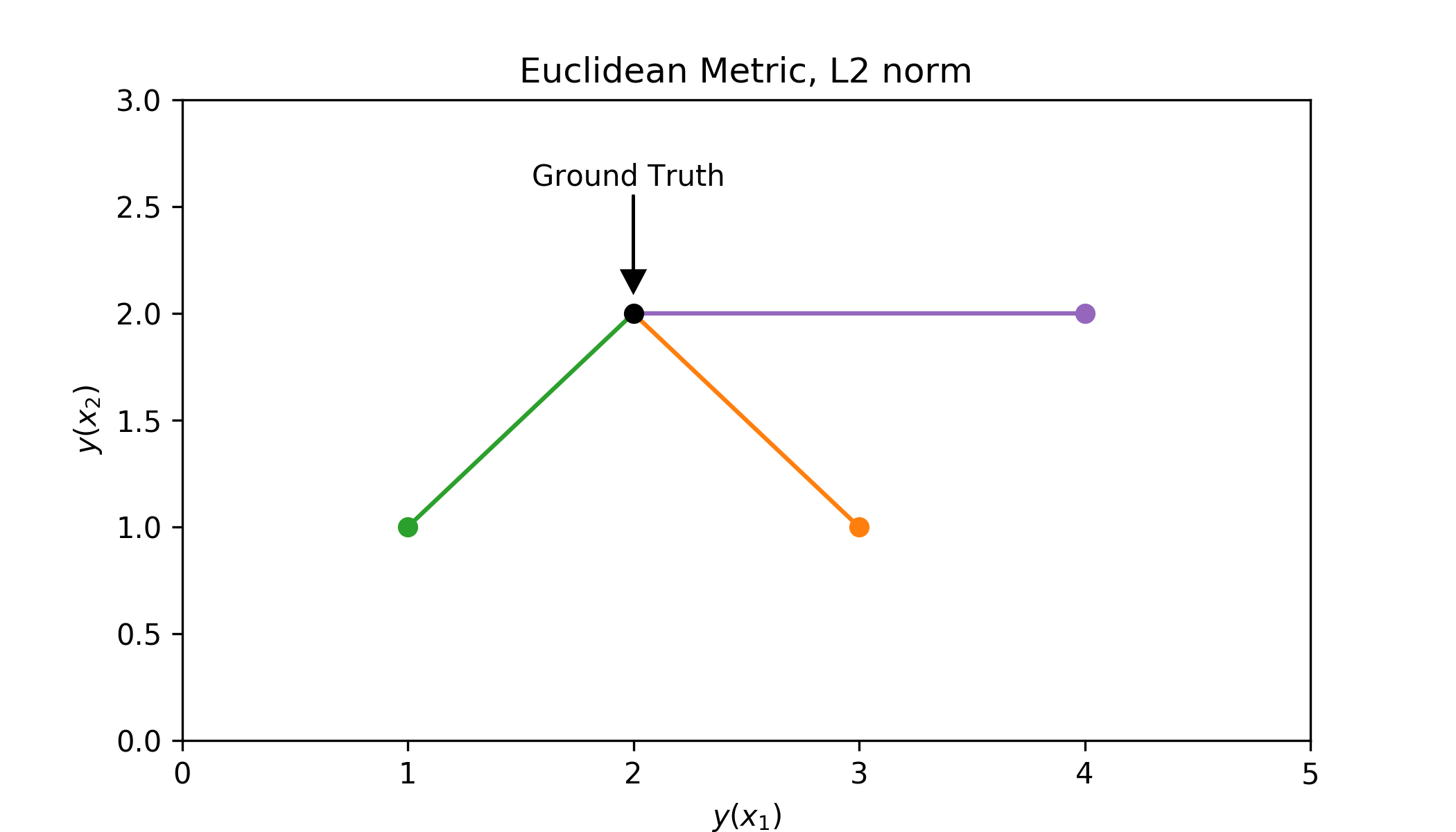
This is achieved by squaring the error instead of using the absolute value (hence the L2-norm). So we modify equation \ref{eq:mae} to be \begin{equation*} L(\theta) = \frac{1}{N}\sum_n^N \delta(x_n; \theta)^2 \end{equation*}
Note that this is not exactly the euclidean distance, as there is no square root. You can drop it as the characteristics are approximately the same, yet computational efficiency is gained. Adding the square root would give us another loss function called Root Mean Squared Error. Since mean squared error and root mean squared error are tightly related you can throw them into the same bag and we will not discuss them separately. Root mean squared error benefits from a more interpretable value, as it is in the same domain as the outputs.
Knowing how to calculate the distance we can use it to again compare the toy examples.
| model | prediction | L2 norm$^2$ |
|---|---|---|
| perfect | $(2, 2)$ | $0$ |
| green | $(1, 1)$ | $2$ |
| orange | $(3, 1)$ | $2$ |
| purple | $(4, 2)$ | $4$ |
With this measure, the purple model is considered worse than the rest. This is because the euclidean distance punishes individual differences more than does the taxicab metric. This is the most important difference between the two loss functions and its consequences will be discussed later.
Before we move on, again we want to know how to find a better model and this is possible using gradient descent, so we calculate the gradient: \begin{equation*} \frac{\partial L(\theta)}{\partial \theta} = \frac{2}{N} \sum_{n=1}^N \delta(x_n; \theta)\frac{\partial \hat{y}}{\partial \theta} \end{equation*} Now the gradient is continuous! It also decreases when it is closer to the minimum making it not only computationally more efficient but easier to converge! The traces of the loss function and it’s derivative are shown on the figure below.
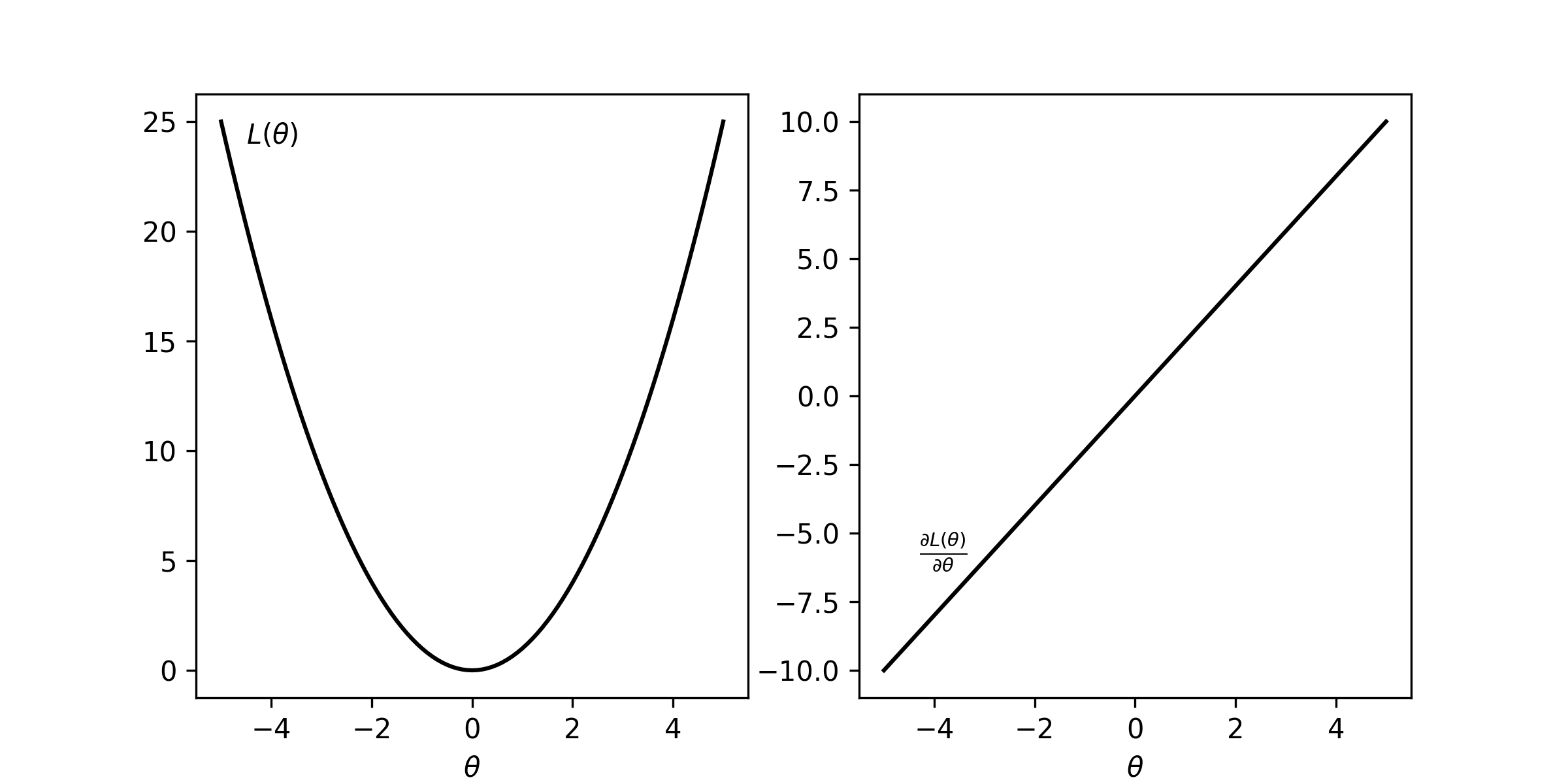
The python implementation as a result is even simpler. Note that we drop the 2 in the gradient as it can be accounted for in the learning rate (see: gradient descent).
1
2
3
4
5
def mse(y_pred, y_true):
    return np.mean((y_pred - y_true)**2)

def mse_grad(y_pred, y_true, y_pred_grad):
    return np.mean((y_pred - y_true) * y_pred_grad)
You can again play around with a demo, which this time uses the mean squared error. Can you see any differences in the fits?
Influence of outliers
A question may arise whether there is any reason to use mean absolute error over mean squared error. After all, the mean squared error is computationally more efficient, and they give the same results. The difference is in the way that outliers are treated. The underlying goals of the two loss functions differ slightly. The mean absolute error wants to minimize the distance to all the points equally. This means that it doesn’t prioritize any data point over another. As a result, it will prefer fitting well to most of the points instead of all of them. Mean squared error on the other hand prioritizes distant points. This means it will look for a solution which is closest to all the points.
If we introduce an outlier to the dataset we will observe that the solution given by the mean absolute error doesn’t change, while the solution for the mean squared error shifts in the direction of the outlier. This can be observed in the figure below.
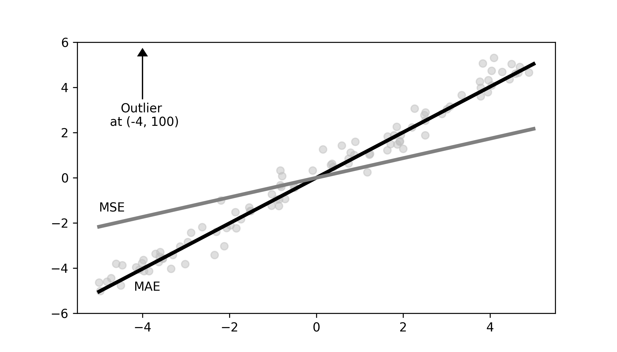
Now whether the behaviour of mean absolute error is good or not depends on what you want to achieve. If you want to be robust against outliers than you might want to use mean absolute error. However, if you are ok with your model including outliers then mean square error would be your choice.
Below you will find another interactive demo. By changing the outlier slider you can observe a shift in the minimum of the mean squared error (grey) loss function.
Conclusion
In essence, you should remember that a loss function defines the objective that you want to obtain and tells you how to reach it. It is important to know what the actual goal of the loss function is to correctly assess, whether it aligns with your objectives. These are not all of the available loss functions, but hopefully based on this article it will be easier for you to understand them. In the future, we will explore some of the other loss functions and their applications in machine learning like linear regression or neural networks.
If you found this article helpful, share it with others so that they can also have a chance to find this post. Also, make sure to sign up for the newsletter to be the first to hear about the new articles. If you have any questions make sure to leave a comment or contact me directly.
Want more resources on this topic?
Citation
Cite as:
Pierzchlewicz, Paweł A. (Sep 2020). What is a Loss Function?. Perceptron.blog. https://perceptron.blog/loss-functions-regression/.
Or
@article{pierzchlewicz2020lossfunctionsregression,
  title   = "What is a Loss Function?",
  author  = "Pierzchlewicz, Paweł A.",
  journal = "Perceptron.blog",
  year    = "2020",
  month   = "Sep",
  url     = "https://perceptron.blog/loss-functions-regression/"
}
